


Thomas Bayes > Quantifying Our Beliefs
More than 250 years ago, Thomas Bayes devised a simple yet powerful rule for updating beliefs when new information arrives. Bayes never saw his famous theorem in print; his friend Richard Price edited and presented the essay posthumously to the Royal Society in 1763. His 18th-century insight — combining your “prior” hunch with the strength of fresh evidence — still underpins everything from Microsoft’s first Bayesian spam filter to Netflix’s recommendation algorithms and modern medical-diagnostic tools. Even in 2018, the University of Edinburgh opened a £45 million “Bayes Centre” to drive cutting-edge data-science research - proof that an 18th-century idea still powers 21st-century innovation.
The Problem: One-Shot Thinking
All too often, we settle on the first story or explanation that pops into our heads and never look back. Imagine you blew a job interview and immediately conclude, “I’m too inauthentic to compete.” Or you find a parking ticket on your windscreen and think, “That traffic warden must have had it in for me.”
This snap-judgement style — what I’ll call one-shot thinking — ignores the fact that a single outcome often has multiple plausible explanations. By jumping to our first explanation, we invite errors, self-criticism and blind spots into our reasoning.
Cognitive Bias Primer
Before we learn how to weigh alternatives, let’s meet three mental shortcuts that steer us off course:
Anchoring
We cling to the first figure or idea we hear.If someone mentions a salary of £30 000, every later offer feels high or low compared to that anchor — even if the true range is £35–45 000.
Availability
We judge how common an event is by how easily examples come to mind.After watching a news story about a plane crash, you might overestimate the danger of flying — despite its safety record.
Confirmation Bias
We notice only the facts that back our favourite theory and ignore the rest.If you believe your colleague dislikes you, you’ll remember the one curt reply and glaze over the five friendly chats.
Pause for a moment: which of these biases sounds most familiar in your own life? By spotting them early, you can force yourself to ask, “What else might explain this?”
From One-Shot Judgements to Echo Chambers
Social media algorithms

Modern social-media algorithms actively exploit these same biases by curating our feeds to match our existing preferences, creating so-called “filter bubbles” that reinforce our initial assumptions. This personalised curation narrows the range of perspectives we see, intensifying confirmation bias and deepening echo chambers (Pariser, 2011; Zollo & Quattrociocchi, 2017). Research studies show that algorithmic ranking dramatically reduces exposure to counter-attitudinal content, making it harder to encounter — and therefore consider — alternative explanations (Bakshy, Messing, & Adamic, 2015; Nikolov et al, 2015). Even when we follow a diverse set of sources, ranking engines still prioritise familiar narratives, steepening the walls of our mental echo chambers. As a result, our feeds become a steady stream of agreeable viewpoints — much like a pleasurable fix — making it ever more difficult to step back, question our first impressions, and update our beliefs objectively (Pariser, 2011).
Enter… Bayesian inference!
Bayes’ Theorem: Posterior, Evidence & Prior
Before we run through a concrete example, let’s label each piece of Bayes’ rule in plain English. Note that the ‘P’s in the formula are probabilities or likelihoods ranging from 0 to 1. We can also understand these Ps as degrees of confidence in our hypotheses or beliefs (H). For example, if P (H) is 1.0, then we know this hypothesis H with certainty - e..g P(H) = 1 if H is ‘2+2=4’.
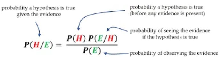
The Prior (P (H))
Your initial belief about how likely hypothesis H is, before seeing any new evidence.
The Evidence / Likelihood (P (E | H))
How likely you would be to observe the evidence E if hypothesis H were true. This is a ‘conditional probability’ - how probable is the data assuming the hypothesis is true))The Normaliser (P (E))
The overall chance of seeing that evidence E under all possible hypotheses — essentially a rescaling factor so that your updated beliefs add up to 100 %.The Posterior (P (H | E))
Your updated belief in hypothesis H after taking the evidence E into account.
In many practical discussions — especially when comparing multiple hypotheses—the denominator P(E) is understood as the scaling factor and dropped from notation. You’ll commonly see Bayes’ theorem written as::
You can also call this Bayes’ theorem — the heart of Bayesian reasoning that turns your prior beliefs and new evidence into updated, coherent levels of confidence in your updated beliefs in the light of evidence. This captures the core ideas of this type of fluid intelligence based reasoning.
Iceland Weather Example
Imagine you’re on holiday in Reykjavík and you check the forecast the night before:
Prior P (H)
The weather app forecasts a 70 % chance of rain.Your prior belief (P (rain)) = 0.7 (this is H1)
Your prior belief (P (no rain)) = 0.3 (this is H2)
We are using the Bayes rule for both these hypotheses (beliefs), not just one. We apply the rule to use our fliuid intelligence to think analytically about different possible explanations rather than just trusting our initial instincts about what the morning will bring on our holiday. Generating alternatives is super important if we want to be smart.
New Evidence P (H |E)
When you wake up, you look out the window and see clear blue sky with no clouds.How likely is it to see a bright sunny morning if it really will rain later (H1)? Probably low — maybe 20 %. (Think carefully about diagnosics here.)
How likely is it to see a sunny morning if it won’t rain (H2)? Quite high — say 90 %. (Think carefully about diagnosics here too.)
These are your ‘Evidence’ estimates:
P (Evidence | rain) ≈ 0.2
P (Evidence | no rain) ≈ 0.9
Unscaled Scores
Multiply each prior by its likelihood:rain: 0.7 × 0.2 = 0.14
no rain: 0.3 × 0.9 = 0.27
Normaliser
Sum these scores to rescale them into valid probabilities:P (Evidence) = 0.14 + 0.27 = 0.41
Posterior / Updated Belief P(H | E)
Divide each unscaled score by the normaliser (you could use your phone calculator for this):P (rain | sunny morning) = 0.14 ÷ 0.41 ≈ 0.34 (34 %)
P (no rain | sunny morning) = 0.27 ÷ 0.41 ≈ 0.66 (66 %)
Why compare?
Because we’ve now computed a posterior probability for each of our two hypotheses, we can directly see which one the evidence supports more strongly. In this case, a sunny morning makes “no rain” nearly twice as likely as “rain,” so we can be most confident in the no-rain hypothesis.
What has been inferred?
Even though the forecast said 70 % rain, seeing clear skies this morning makes “no rain” now twice as likely as “rain.” The normaliser (0.41) simply rescales your new scores so they add up to 100 %, giving you coherent updated odds.
So, running through this process, you have a solid rational basis for going out on a hike rather than going to a museum that morning! Trust in the process!
Your Bayesian Mindware
You can use the Bayesian Hypothesis Comparator AI GPT bot I built to run this Bayesian inference method on some of your own alternate hypotheses or possible explanations for an experience, event or data in your life. Use the video tutorial to help you use this:
Bayes Mindware Exercises
For each scenario you can also do some mental arithmetic rather than using the bot - by assigning prior probabilities to your hypotheses (based on background knowledge) and estimate how likely new evidence would occur under each hypothesis (the likelihood).
The more you practice, the easier and more automatic the skill with this mindware becomes.
1. Backward-Looking Explanations
Retrospective explanations often fall prey to hindsight bias, where we latch onto the first story that comes to mind rather than weighing multiple possibilities.
Example 1: A Friend Didn’t Return Your Call
Hypothesis A: They were busy at work and simply forgot.
Hypothesis B: They’re upset with you after your last conversation.
Hypothesis C: Their phone battery died, so they didn’t see the call.
Example 2: Your Keys Have Gone Missing
Hypothesis A: You lent them to a relative and forgot.
Hypothesis B: They slipped out of your pocket at the café yesterday.
Hypothesis C: You accidentally left them at the office desk.
2. Forward-Looking Beliefs
Forecasts about the future often reflect overconfidence in our internal models; Bayesian updating keeps us honest by forcing explicit priors and likelihoods.
Example 1: “I’ll Get That Promotion”
Model A: Your performance review was stellar, boosting your odds.
Model B: The company seldom promotes more than one person per year.
Model C: A recent reorganisation could delay all promotions.
Example 2: “My New Plant Will Survive”
Model A: It’s a hardy species with a 90 % survival rate under similar care.
Model B: You’ve been inconsistent with watering, reducing chances to about 50 %.
Model C: Recent pests in your area make survival only 30 %.

